Tensorboard: What and why

TensorBoard is a visualization tool, which can demonstrate model related details as model being trained. It can be running on both browser and Jupyter Notebook.

Given the high time consumption of the deep neural network training nowadays, the monitor of model training is a good feature to have to let researchers to understand and tune the training processes. For example. one can decide if we need to continue to train model by looking at loss versus epoch curve, and study evolution of the parameters on one specific layer by checking parameters versus epoch plot, etc.. Moreover, one can also compare the training processes from different models by checking the monitoring results. Tensorboard is a visualization tool that satisfy these scenarios.

In TensorBoard, one can monitor scalar (loss, accuracy, etc.) evolution along with epoch, check model parameters distribution and histogram evolution along with epoch, view model graphs, and other self-defined features that written into TensorBoard logs. etc.. All these features will be demonstrated with code snippets in next section.

Visualize Tensorflow model training with TensorBoard

In this section, both default features that already defined in TensorBoard callback function and self-defined features that customized by user are demonstrated as model training monitoring.

Pre-training setup

First, Let’s build a simple neural network to train MNIST dataset:

import datetime
import os

import numpy as np
import tensorflow as tf

# Dataset loading
(train_image, train_label), (test_image, test_label) = tf.keras.datasets.mnist.load_data()

# Dataset engineering
train_image = tf.cast(tf.expand_dims(train_image, -1)/255, tf.float32)
train_label = tf.cast(train_label, tf.int64)
test_image = tf.cast(tf.expand_dims(test_image, -1)/255, tf.float32)
test_label = tf.cast(test_label, tf.int64)

train_dataset = tf.data.Dataset.from_tensor_slices((train_image, train_label))
train_dataset = train_dataset.repeat().shuffle(60000).batch(128)
test_dataset = tf.data.Dataset.from_tensor_slices((test_image, test_label))
test_dataset = test_dataset.repeat(1).batch(128)

# Model building
model = tf.keras.Sequential([
    tf.keras.layers.Conv2D(16, [3,3], activation='relu', input_shape=(28, 28, 1)),
    tf.keras.layers.Conv2D(32, [3,3], activation='relu'),
    tf.keras.layers.GlobalMaxPool2D(),
    tf.keras.layers.Dense(10, activation='softmax'),
])

model.compile(
    optimizer=tf.keras.optimizers.Adam(),
    loss=tf.keras.losses.SparseCategoricalCrossentropy(),
    metrics=['accuracy'],
)

With the model defined and compiled, one need to define callback functions to get monitoring data before starting to train the model. The fit function of model object will take these callback functions as input parameter, and call it at each epoch. The output data will be written into a directory. To be more organized in log, I integrate the timestamp together with the directory name:

log_dir = os.path.join('logs', datetime.datetime.now().strftime("%T%m%d-%H%M%S"))

Default features in Tensorboard

To obtain monitoring features that already defined in the Tensorflow callback functions, one can define the tensorboard_callback:

tensorboard_callback = tf.keras.callbacks.TensorBoard(log_dir=log_dir, histogram_freq=1)

Self-defined features in Tensorboard

One can also defined his own callback function to monitoring whatever feature he/she want to monitor. This callback function needed to be able to write data into log directory. SummaryWriter is the class, which can be instantiated by create_file_writer, to write monitoring data into log directory, For example, if one want to have a smaller learning rate when training on more epochs, and monitor that learning rate along with epoch, the callback function could be:

file_writer = tf.summary.create_file_writer(log_dir+'/lr')
file_writer.set_as_default()

def lr_sche(epoch):
    lr = 0.2
    if epoch > 5:
        lr = 0.02
    if epoch > 10:
        lr = 0.01
    if epoch > 20:
        lr = 0.005
    tf.summary.scalar('learning_rate', data=lr, step=epoch)
    return lr

lr_callback = tf.keras.callbacks.LearningRateScheduler(lr_sche)

NOTE: Forgive my messy implementation. To write a decent customized callback function class, please refer to official Tensorflow callback class.

Model training and monitoring

Once callback functions have been defined, one can put it into model fit parameter to enable monitoring:

model.fit(
    train_dataset,
    epochs=25,
    steps_per_epoch=60000//128,
    validation_data=test_dataset,
    validation_steps=10000//128,
    callbacks=[tensorboard_callback, lr_callback],
)

Once model training complete, we can start monitoring service either in browser from terminal:

tensorboard --logdir logs/

or in Jupyter notebook with code block:

%load_ext tensorboard
%matplotlib inline
%tensorboard --logdir logs/

. User interface will pop out after commands above executed.

The default scalar, like loss and accuracy both train data and validation data looks like:

. From this plot, we can see that the loss does not decrease too much after epoch 12, and validation accuracy is lower than train accuracy, which imply a more complicated model is needed to improve the accuracy.

And self-defined scalar, learning rate, can be monitored:

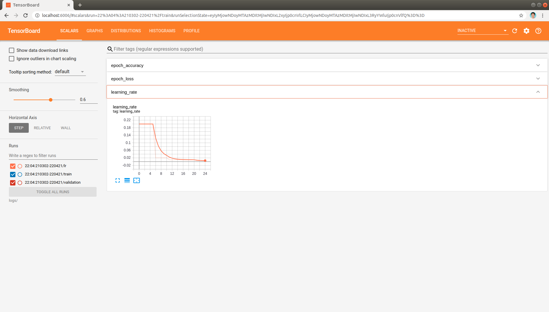
, which indicates that the learning rate is changed as expected when training epoch increased.

Moreover, the distribution and histogram of model parameters are demonstrated like:

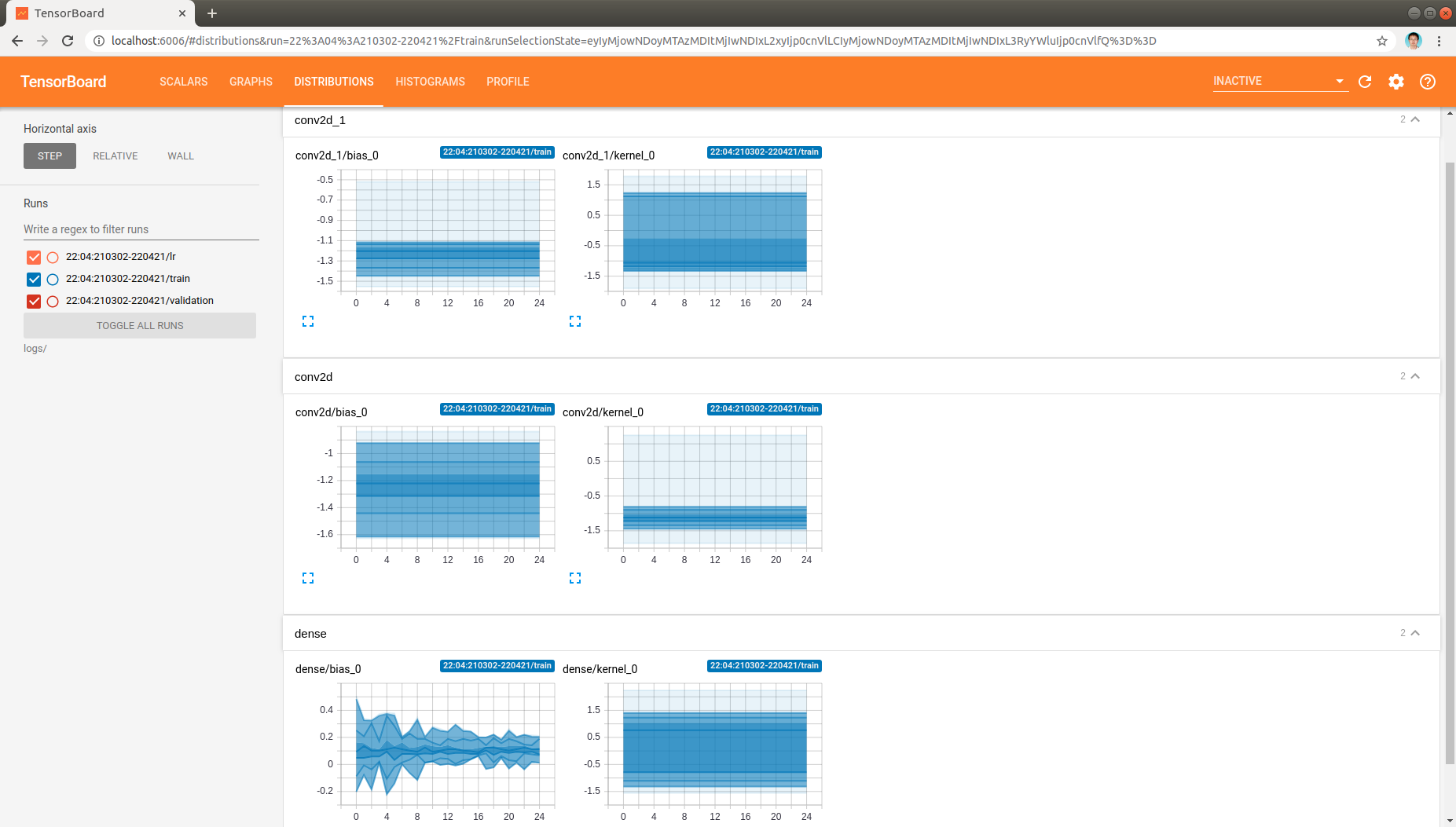
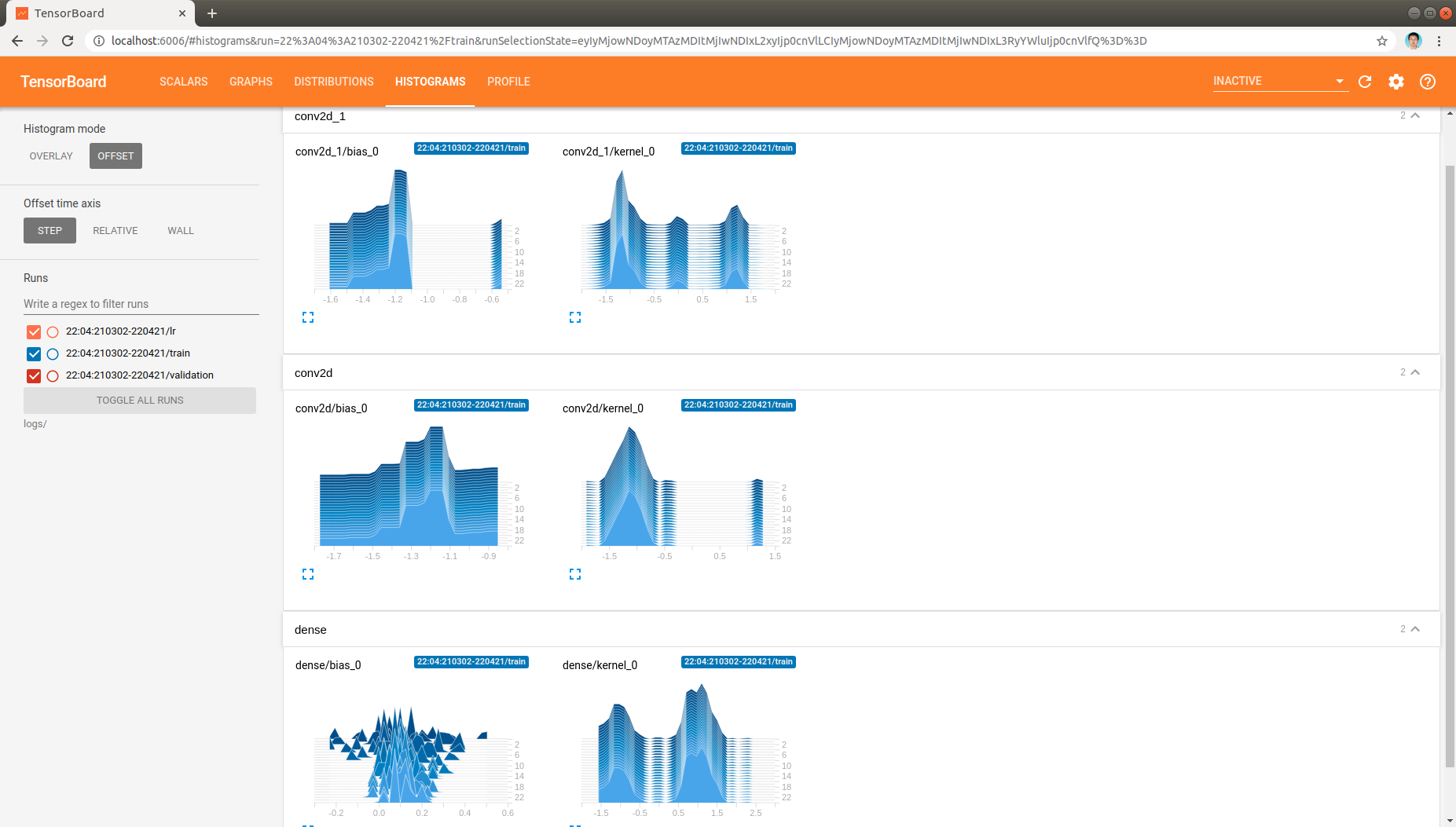
, which demonstrate the model parameters in all layers as model being trained.

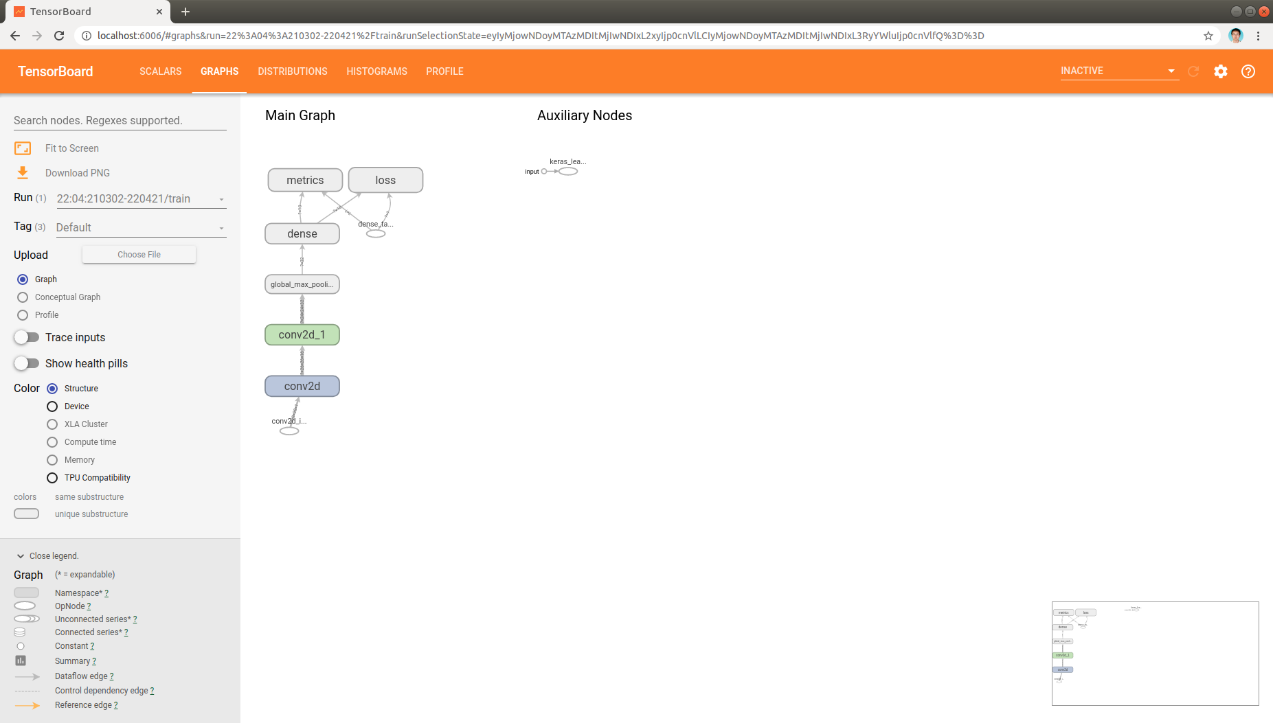
Finally, the model architecture can be found in graph tab also:

Trouble shooting

In case of missing data in display or other issues, one can use the following command to investigate the TensorBoard data that saved in the log directory:

tensorboard --inspect --logdir logs/

More readings

• TensorBoard guide in Tensorflow