What is Hash table
A hash table is a data structure that implements an associative array that can map keys to values. A hash table uses a hash function to compute index from the key, which can be referred directly as the location of the value stores. Ideally, the hash table data structure can provide O(1) time complexity to insert, get, update and delete value by key.
However, hash table can only achieve desired performance given a perfect hash function, which indicates that different keys are not mapped to same index. On other side, the range of output of hash function should be limited, since system have limited amount of memory. As a result, it is not trivial to design a hash function with both low collision rate and high load factor (Number of entries in hash table / Number of buckets allocated).
Once hash function is determined, another issue need to be resolved is collision. Collision happens when two different keys have same output, which indicate same “physical” location. One need to find a way to resolve this collision, otherwise, the output value maybe wrong given a key as input.
Hash function
A good hash function must satisfy the following criteria:
- Fast enough to compute: Small CPU cost.
- The outputs of hash function are uniformly distributed: Reduce collisions.
Given the first criteria, all cryptographic hash functions, like SHA1, MD5, etc., are not good candidate, because they are designed to be hard to reverse, therefore relatively costly in computation. The second criteria is hard to guarantee by hash function itself. The uniformity can be tested by statistical test, for example, Pearson’s Chi-Squared test for discrete uniform distribution.
One can us SMHasher dataset to benchmark hash function. One of the most popular hash function is called MurmurHash. More details of non cryptographic hash functions can be found in more readings section.
Collision resolution
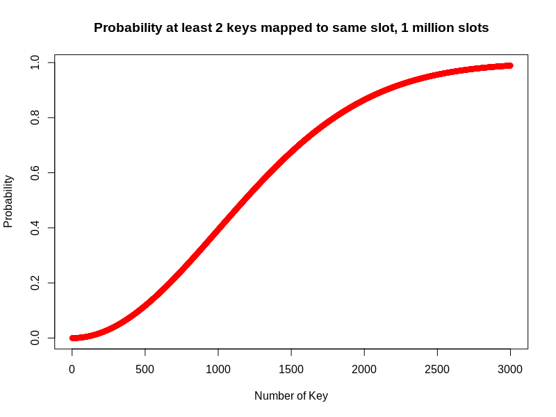
Collisions are practically unavoidable when hashing a large set of keys. The collision probability estimation can be interpreted as a statistical problem: Given m keys, and n memory blocks (m < n), estimate the probability that at least two keys take same slot. This is very similar to Birthday problem. The probability distribution of number of keys in case of 1 million slots can be viewed in the figure below:

As we can see, the probability to have at least 1 collision for 1 million slots are more than 95% when number of keys is 2500. The plot can be easily generated by the following R code snippet:
nKey = 3000
nSlot = 1000000

calcHashCollisionProb <- function(m, n) {
    outArr <- numeric(m)
    for (i in 1:m) {
        q <- 1 - (0:(i - 1))/n # 1 - prob(no matches)
        outArr[i] <- 1 - prod(q)
    }
    return(outArr)
}

arr <- calcHashCollisionProb(nKey, nSlot)
plot(arr, main="Probability at least 2 keys mapped to same slot, 1 million slots", xlab ="Number of Key", ylab = "Probability", col="red")
As a result, one must resolve the hash function collisions when implement hash table. Separate Chaining and Open Address are two basic ideas to resolve the collision issue.
Separate Chaining
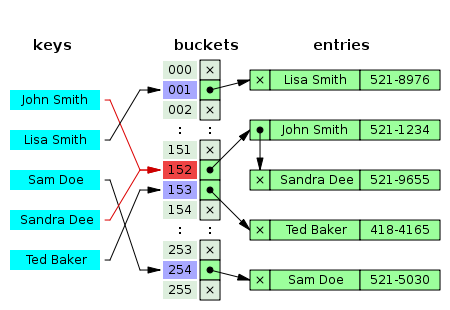
In separate chaining approach, all buckets are independent, and collided keys are attached on same bucket as a list. As shown in the figure, “John Smith” and “Sandra Dee” are mapped onto same bucket. The key “John Smith” and its value come first and attached directly onto bucket. “Sandra Dee” and its value come later and attached after “John Smith” pair. As a consequence, one have to loop over the linked list in case of collision to find out correct value. Moreover, linked list structure also caused discrete space allocation.

Open Addressing
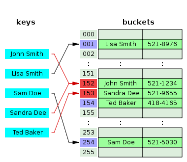
The open addressing approach, on the other hand, try to map keys to sparse distributed buckets, which means empty slots left in between. These empty slots are designed to resolve collision. In the example shown in the figure, Key “John Smith” and “Sandra Dee” map onto same bucket. “Sandra Dee” pair find key “John Smith” already occupied the bucket 152, therefore, it will try to find next available bucket to sit in, which is bucket 153. The procedure of searching next available bucket is called “probe sequence”. One of the most commonly used probe sequence is linear probe, which means searching for available bucket by increment id 1 until found. It is obvious that the performance of probe sequence can be quite bad in case of high load factor.

Examples
In this section, several examples are given to implement associative array with hash table. Note that not all associative array are implemented with hash table, for example. map and set in C++ STL are used red-black tree as its basis. However, in order to achieve O(1) time complexity, hash table is the best data structure to use (unordered_set and unordered_map).
Java jdk7u6-b07, HashMap
The HashMap, in OpenJDK 7, is a hash table based associative array. The separate chaining approach is applied to resolve collision. In the HashMap class, addEntry method, one add new entry as the head of linked list on the bucket ID, and all existed nodes move after the newly added one.
    /**
     * Adds a new entry with the specified key, value and hash code to
     * the specified bucket.  It is the responsibility of this
     * method to resize the table if appropriate.
     *
     * Subclass overrides this to alter the behavior of put method.
     */
    void addEntry(int hash, K key, V value, int bucketIndex) {
        Entry<K,V> e = table[bucketIndex];
        table[bucketIndex] = new Entry<>(hash, key, value, e);
        if (size++ >= threshold)
            resize(2 * table.length);
    }
Python 3.6, dict
The dict is a widely used data structure in python, not only in python package, but also in cpython interpreter. The dict is actually an associative array, based on hash table. Python dict is using open addressing approach to resolve collision, as shown in code block Python3.6, dictobject.c, L662-799.
/*
The basic lookup function used by all operations.
This is based on Algorithm D from Knuth Vol. 3, Sec. 6.4.
Open addressing is preferred over chaining since the link overhead for
chaining would be substantial (100% with typical malloc overhead).
The initial probe index is computed as hash mod the table size. Subsequent
probe indices are computed as explained earlier.
All arithmetic on hash should ignore overflow.
The details in this version are due to Tim Peters, building on many past
contributions by Reimer Behrends, Jyrki Alakuijala, Vladimir Marangozov and
Christian Tismer.
lookdict() is general-purpose, and may return DKIX_ERROR if (and only if) a
comparison raises an exception.
lookdict_unicode() below is specialized to string keys, comparison of which can
never raise an exception; that function can never return DKIX_ERROR when key
is string.  Otherwise, it falls back to lookdict().
lookdict_unicode_nodummy is further specialized for string keys that cannot be
the <dummy> value.
For both, when the key isn't found a DKIX_EMPTY is returned. hashpos returns
where the key index should be inserted.
*/
static Py_ssize_t
lookdict(PyDictObject *mp, PyObject *key,
         Py_hash_t hash, PyObject ***value_addr, Py_ssize_t *hashpos)
{
    size_t i, mask;
    Py_ssize_t ix, freeslot;
    int cmp;
    PyDictKeysObject *dk;
    PyDictKeyEntry *ep0, *ep;
    PyObject *startkey;

top:
    dk = mp->ma_keys;
    mask = DK_MASK(dk);
    ep0 = DK_ENTRIES(dk);
    i = (size_t)hash & mask;

    ix = dk_get_index(dk, i);

    // Hua Wei's comment: if the index not occupied, take it directly, exit.
    if (ix == DKIX_EMPTY) {
        if (hashpos != NULL)
            *hashpos = i;
        *value_addr = NULL;
        return DKIX_EMPTY;
    }
    if (ix == DKIX_DUMMY) {
        freeslot = i;
    }
    else {
        ep = &ep0[ix];
        assert(ep->me_key != NULL);
        if (ep->me_key == key) {
            *value_addr = &ep->me_value;
            if (hashpos != NULL)
                *hashpos = i;
            return ix;
        }
        if (ep->me_hash == hash) {
            startkey = ep->me_key;
            Py_INCREF(startkey);
            cmp = PyObject_RichCompareBool(startkey, key, Py_EQ);
            Py_DECREF(startkey);
            if (cmp < 0) {
                *value_addr = NULL;
                return DKIX_ERROR;
            }
            if (dk == mp->ma_keys && ep->me_key == startkey) {
                if (cmp > 0) {
                    *value_addr = &ep->me_value;
                    if (hashpos != NULL)
                        *hashpos = i;
                    return ix;
                }
            }
            else {
                /* The dict was mutated, restart */
                goto top;
            }
        }
        freeslot = -1;
    }

    // Hua Wei's comment: if the index occupied (freeslot = -1), shift until empty found.
    for (size_t perturb = hash;;) {
        perturb >>= PERTURB_SHIFT;
        i = ((i << 2) + i + perturb + 1) & mask;
        ix = dk_get_index(dk, i);
        if (ix == DKIX_EMPTY) {
            if (hashpos != NULL) {
                *hashpos = (freeslot == -1) ? (Py_ssize_t)i : freeslot;
            }
            *value_addr = NULL;
            return ix;
        }
        if (ix == DKIX_DUMMY) {
            if (freeslot == -1)
                freeslot = i;
            continue;
        }
        ep = &ep0[ix];
        assert(ep->me_key != NULL);
        if (ep->me_key == key) {
            if (hashpos != NULL) {
                *hashpos = i;
            }
            *value_addr = &ep->me_value;
            return ix;
        }
        if (ep->me_hash == hash) {
            startkey = ep->me_key;
            Py_INCREF(startkey);
            cmp = PyObject_RichCompareBool(startkey, key, Py_EQ);
            Py_DECREF(startkey);
            if (cmp < 0) {
                *value_addr = NULL;
                return DKIX_ERROR;
            }
            if (dk == mp->ma_keys && ep->me_key == startkey) {
                if (cmp > 0) {
                    if (hashpos != NULL) {
                        *hashpos = i;
                    }
                    *value_addr = &ep->me_value;
                    return ix;
                }
            }
            else {
                /* The dict was mutated, restart */
                goto top;
            }
        }
    }
    assert(0);          /* NOT REACHED */
    return 0;
}
Golang 1.14, map
The map is a hash table based associative array in Golang. It also applies separate chaining approach to resolve collision. However, it uses a data structure called bmap with 8 slot, each slot can serve for one key-value pair. This bmap also contains a overflow object, which indicate the next bmap in the bucket. The map data structure uses first 8 bits of hashed index as top hash to find the location inside bmap, and uses 4 bits to find out bucket ID. These two layers buckets structure can speed up the collision resolution. One can check more details in Golang1.14, runtime, hmap.
Conclusion
In this blog, the hash table definition, including hash function and collision resolution are described briefly. Several real world examples that using hash table are demonstrated in detail. More advanced topic, like hash function design, advanced collision resolution, capacity resize, distributed hash table, etc, will be covered in other articles.